The Dangers of Monte Carlo Simulations
Membership required
Membership is now required to use this feature. To learn more:
View Membership Benefits Advisor Perspectives welcomes guest contributions. The views presented here do not necessarily represent those of Advisor Perspectives.
Probability-based retirement income strategies are highly sensitive to the capital market assumptions used in Monte Carlo analysis. Seemingly small changes in those assumptions can mean the difference between projecting a comfortable lifestyle and financial ruin.
Many advisors use Monte Carlo analysis to evaluate withdrawal strategies for their retired clients. Using their financial planning tools, advisors calculate the “probability of success” of a given withdrawal strategy; if the probability is high enough, advisors may feel comfortable communicating that the plan is “safe.”
However, the results of Monte Carlo analysis depend heavily on the capital market assumptions (CMAs) used. It may seem that running thousands of Monte Carlo simulations is “scientific,” showing what would happen to a portfolio under all possible future scenarios.
But it is not.
The results from Monte Carlo are entirely determined by the CMAs used.
In this article, we evaluate the sensitivity of “safe” withdrawal rates and probability of success metrics to different CMAs, using a recent survey of investment firms’ CMAs. Our findings suggest that unless advisors are confident that they are using highly accurate CMAs, probability of success metrics will mislead clients into a false sense of security.
The standard model: Probability-based retirement income
We use the following example for our analysis in this article.
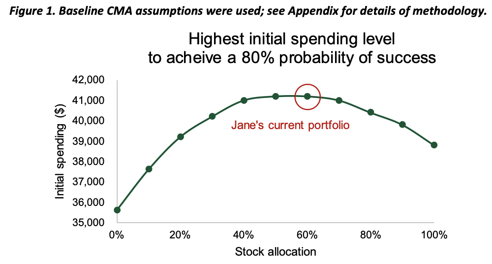
Jane is 65 and just retired. She has $1 million in an IRA, and her current allocation is 60% U.S. large-cap stocks and 40% U.S. investment-grade corporate bonds. She works with her advisor to arrive at a prudent portfolio and withdrawal strategy to make sure she does not run out of money by age 95.
The advisor uses a planning tool to run 1,000 Monte Carlo simulations, evaluating different withdrawal rates as well as different portfolios for Jane. Standard practice at the advisor’s firm is to use 80% probability of success as the cutoff – anything less than that is not considered “safe enough.” The results show that if Jane keeps her current portfolio, she can spend $41,200 next year, and 2% more each year after that to adjust for inflation, with an 80% probability of success to age 95.
This result is roughly consistent with the “4% rule” used by many advisors, which Jane may have heard of. She goes home confident in her plan and reassured that it is “safe.”
Monte Carlo unmasked
Is Jane right to feel secure in this answer?
“Monte Carlo analysis” and “probability of success” sound like highly technical and scientific terms. But what’s behind the math?
Probability of success is the percentage of Monte Carlo simulations where the client a) spends a given amount each year and b) still has money left over at a given age. An 80% probability of success means that in 80% of simulations, Jane still has money at age 95; in 20% of simulations, she runs out of money before age 95.
Probability of success, therefore, depends on how the Monte Carlo analysis is set up. Monte Carlo is a technique for generating a set of future scenarios (“simulations”). In the case of retirement income, the analysis generates, say, 1,000 simulations of a portfolio, given a withdrawal strategy. But it is not all possible future values, or even a completely “random” selection of future values. The set of future values evaluated is determined entirely by the assumptions fed into the analysis.
In each year of a simulation, the Monte Carlo analysis will assign a return to the portfolio: “the return in year 1 will be X%.” This X% is selected randomly from a pre-determined, specific distribution of returns of the portfolio. But the distribution itself is not random. The distribution is determined by the assumed returns, volatilities, and correlations among asset classes (CMAs). For example, if the average return in the distribution of portfolio returns is 7%, there will be a much higher chance that 7% (or something close to it) is selected as the X% rather than, say, 60% or -15%.
The four types of assumptions that drive the results in Monte Carlo are:
- Returns: Average return forecasts for each asset class, e.g., how much will U.S. large-cap stocks return in the future?
- Volatilities: Volatility of return forecasts for each asset class, e.g., how much will U.S. large cap stock returns vary year to year, on average?
- Correlations: How will the returns of different asset classes be related, e.g., will they tend to both have positive returns at the same time? Or are they negatively correlated?
- Distribution: What the shape of the return distribution will be, e.g., normal distribution, lognormal, etc.; i.e., the specific shape of the bell curve.
Since these are all forecasts, Jane might reasonably ask her advisor: What if you’re wrong?
Who has a crystal ball?
Horizon Actuarial Services is an actuarial consulting firm that surveys major investment firms on their CMAs each year. The latest survey was published in August 2022.

The survey provides the average CMAs across investment firms, as well as the variability in assumptions used by different investment firms. For example, the 20-year return assumptions for stocks and bonds vary significantly across firms:

Using the variability in CMAs in the 2022 Horizon survey, we can start to answer Jane’s question. Depending on which CMAs are used – all from credible investment firms – Jane’s advisor might give her drastically different answers. To know the “right” answer, her advisor would need to know who has the crystal ball.
The following chart shows initial spending levels for different stock return assumptions, keeping all the other assumptions constant (stock volatility, bond returns and volatility, and correlation).
 The results suggest that, given her allocation, the “safe” spending level could be anywhere between $33,000 and over $51,000, just depending on which stock return assumption is used (and keeping everything else the same).
Put differently, if her advisor plays it safe and uses the lowest return prediction, Jane could be underspending by 56% (if the highest return forecast turns out to be the right one). Alternatively, if her advisor aligns with the most bullish forecast, she may be overspending by 36% and have a good chance of running out of money early (if the lowest return forecast turns out to be right).
Another way to look at this is to evaluate the 4% rule in the context of different CMAs. What is the probability of success of the 4% rule using the different return forecasts?

Using the most bullish estimate, Jane’s probability of success using the 4% rule would be over 95%. Using the most pessimistic, it would be just 62%.
But smaller differences matter too. If Jane’s advisor used 7.11% (25th percentile) instead of 8.52% (75th percentile) for stock returns, Jane’s probability of success would fall from 87% to 78%. Put differently, her estimated probability of failure – running out of money completely by age 95 – would increase from 13% to 22%. That’s a 70% higher chance of failure, just based on a return difference of 1.4 percentage points. And that’s just for one input into the Monte Carlo analysis.
Our results (see Appendix I for full details) suggest that probabilities of success, and more generally “safe” withdrawal rates based on Monte Carlo analysis, depend heavily on the accuracy of CMAs. Even relatively small errors in the inputs – 1 or 2 percentage points – will generate meaningful differences in what advisors might consider a “safe” withdrawal strategy.
What can advisors do?
It’s possible that using the average or median of different investment firms’ CMAs may lead to more accurate forecasts. The “wisdom of the crowd” has proven true in other cases. However, our results still imply that if the average CMA is off, even by relatively small amounts, it will significantly impact recommendations given to retirees.
For advisors who can modify the CMAs within their Monte Carlo tool, one remedy could be to stress-test the portfolio by changing the CMAs. Specifically, advisors could use some combination of:
- Lower returns than baseline assumptions;
- Higher volatilities than baseline;
- Higher (more positive) correlations than baseline;
- Higher safety thresholds for probability of success; and
- Longer time horizon / life expectancy assumptions.
While there is no clear answer for how to choose an appropriate level of stress (or, more generally, which CMAs to use), showing more dire assumptions may prevent bad outcomes for clients and give them more comfort that their plan will not turn out disastrously. On the other hand, using more dire CMAs may exacerbate the problem of underspending – if the prediction turns out to be too extremely pessimistic, clients will live well below their means and leave behind more than they might have intended.
As an alternative to this approach, advisors could consider other ways to generate retirement income that do not rely so heavily on forecasts of returns, volatilities, and correlations.
Murguia and Pfau have described different retirement income styles, of which the total return approach relies most heavily on identifying a “safe” withdrawal rate from a diversified investment portfolio. But there are other options, such as the time-segmentation approach or the income-flooring approach, which rely on contractual protections like bond ladders and fixed annuities to secure cash flow. While these approaches have their pros and cons, they do have the advantage of not relying as much on forecasts of future returns.
Wade D. Pfau, Ph.D., CFA, RICP®, is the program director of the Retirement Income Certified Professional® designation and a Professor of Retirement Income at The American College of Financial Services in King of Prussia, PA, as well as a co-director of the college’s Center for Retirement Income. As well, he is a Principal and Director for McLean Asset Management and RISA, LLC. He also serves as a Research Fellow with the Alliance for Lifetime Income and Retirement Income Institute. Wade’s latest book is Retirement Planning Guidebook: Navigating the Important Decisions for Retirement Success.
Massimo Young, CFA leads investment solutions and technology for Insight Investment’s Individual Retirement Solutions group. Note: The views expressed in this article are those of the authors are do not necessarily reflect the views of Insight Investment.
Appendix I: Additional results
Below are results for other variations in CMAs. We vary bond returns, volatilities, correlations, and distribution shape, and evaluate the probability of success of the 4% rule for each variation. We also present results for two extreme CMAs: a “pessimistic” view and an “optimistic” view.
- Pessimistic:
- Stock return: minimum, 5.15%
- Stock volatility: minimum, 13.7%1
- Bond return: minimum, 2.42%
- Bond volatility: minimum, 3.00%3
- Correlation: maximum, 0.40
- Optimistic:
- Stock return: maximum, 10.63%
- Stock volatility: maximum, 19.09%2
- Bond return: maximum, 5.82%
- Bond volatility: maximum, 7.35%4
- Correlation: minimum, -0.32
The range between the most pessimistic overall CMA and the most optimistic is very large. For a 60% stock allocation, the probability of success ranges from 58% (pessimistic) to 99% (optimistic).
In general, the variability in return assumptions has a larger impact on probability of success than the variability in volatility assumptions. However, it is worth noting that for high allocation to bonds, the variability in the bond volatility assumption has a large effect (20 percentage point difference for a 100% bond portfolio).
The effect of the variability in correlations was relatively small – except for the minimum assumption, which is strongly negative (minus 0.32) and therefore significantly increases probability of success.
The two specific distributional assumptions we considered – normal and lognormal – do not appear to have a meaningful effect.

Appendix II: Methodology
The CMAs used in this article are from the Horizon Actuarial 2022 Survey of Capital Market Assumptions. There is a public report available online, but most data were provided directly by Horizon Actuarial Services for this research.
Asset classes:
- “Stocks” is represented by the US Equity - Large Cap asset class in the Horizon survey
- “Bonds” is represented by the US Corporate Bonds – Core asset class in the Horizon survey
Baseline CMAs:
The Baseline CMAs are 20-year forecasts. They are the median across respondents in the survey.
- Stock returns: 7.80% (arithmetic)
- Stock volatility: 16.61%
- Bond returns: 3.75% (arithmetic)
- Bond volatility: 6.00%
- Correlation: 0.23
CMA variation:
- Stock returns:
- Min: 5.15%
- 25th percentile: 7.11%
- 75th percentile: 8.52%
- Max: 10.63%
- Stock volatility:
- Min: 13.70%
- 25th percentile: 15.90%
- 75th percentile: 17.25%
- Max: 19.09%
- Bond returns:
- Min: 2.42%
- 25th percentile: 2.80%
- 75th percentile: 4.11%
- Max: 5.82%
- Bond volatility:
- Min: 3.00%
- 25th percentile: 4.40%
- 75th percentile: 6.72%
- Max: 7.35%
- Correlation:
- Min: -0.32
- 25th percentile: 0.02
- 75th percentile: 0.33
- Max: 0.40
Other notes:
- Returns are modeled as lognormally distributed, unless noted otherwise.
- A 30-year time horizon is assumed.
- Portfolio is rebalanced annually to target allocation.
- Withdrawals are assumed to be annual.
- 1,000 simulations are run.
1Although a higher volatility would be more pessimistic, it is likely that the respondent with the lowest return assumption also had the lowest associated volatility.
2Although a lower volatility would be more optimistic, it is likely that the respondent with the highest return assumption also had the highest associated volatility.
Membership required
Membership is now required to use this feature. To learn more:
View Membership BenefitsSponsored Content
Upcoming Virtual Events View All