Pring Turner Approach to Business Cycle Investing
Introduction
The investment strategies utilized by Pring Turner Capital Group at one extreme draws on our assessment of very long-term secular trends in bonds, stocks and commodities; at the other, our stringent risk control strategies. The heart of our investment approach though, focusses on business cycle associated trends for bonds, stocks and commodities and is based on two observations. First, the typical four to five year business cycle consists of a series of chronological events that have continually repeated since the beginning of the industrial revolution over 150 years ago. Second, the optimal asset allocation and sector rotation for investment portfolios can be adjusted based on the stage of the business cycle in an effort to increase returns while reducing risks. The calendar year rotates through four repeatable seasons, the knowledge of which empowers farmers to plant in the spring, harvest in the fall and avoid the problematic cold of winter. Like the seasons of the year, the environment for bonds, stocks, and commodities also changes in a repeatable and sequential fashion. Many investors are unaware of and unprepared for the ever-changing financial market seasons.
What is the business cycle?
Reasonably reliable economic statistics in the U.S. go back to the start of the nineteenth century. Since that time the U.S has observed consistent fluctuations in the level of economic activity between growth and contraction, better known as the business cycle. According to the National Bureau of Economic Research, since 1857 these cycles have averaged 56-months from trough to trough. It would be convenient if the cycle operated on a regular beat and repeated more or less exactly on each occasion, but unfortunately each cycle has its own unique characteristics. That’s because the economy consists of many parts or sectors whose growth paths change from cycle to cycle. For example, in the opening years of the twenty first century housing starts registered monthly annualized levels in excess of 2 million but after the housing bust the post 2009 recovery barely managed to reach 800,000 after three years of progress. Whatever the reason we usually find there is typically one sector of the economy that over-invests, over-builds or over-lends, which causes an increase of its share of the economic pie on the way up and exaggerate the speed of its declining share on the way down.
Another reason for changing business cycle characteristics comes from substantial structural differences that take place over time. The source of such transformations might emanate from demographic make-up, innovation, social trends and so forth. For example, in the early 1800’s the U.S. economy was strongly represented by farmers. Later manufacturing dominated and in the latter part of the twentieth century the service industries came to the fore. The expanding role and influence of federal, state and local governments is another factor. Innovation has meant that principal forms of communication have moved from letters and telephones in the late twentieth century to the internet, email, texting and mobile phones in the second decade of the twenty first and this is just the tip of the iceberg. The one thing that does not change is the fact that the business cycle follows a consistent, rational, and logical sequence of events, which continually provides new investment opportunities.
Why does the business cycle repeat?
The alternation between recovery and recession is a direct function of people responding to positive stimuli (the economic recovery) and subsequently repeating the same mistakes that cause a contraction. These decisions are psychologically driven, either in anticipation of future conditions, or as a response to existing ones. For example, corporations expand their capacity to produce because they anticipate future growth. On the other hand, workers are often laid off in response to declining sales. The essential point to grasp is the business cycle develops because human nature is more or less constant. They say that history repeats but never exactly. The same is true of the business cycle. People make the same mistakes, but each time it is different people in different sectors making mistakes. Put yourself in the same position as a business owner and you will understand why it is so easy to make the same mistakes. If business activity has been contracting and your company is really suffering along with your competitors it is easier to make those cost cutting decisions. On the other hand, if you are certain that the economy is going to pick up next month you would perhaps postpone or cancel the cost cutting exercise. “The regularity is in the pattern of these reactions, not in the cycle itself” is how the late Dr. Richard Coghlan put it in his book (McGraw Hill, London, 1992).
Demonstrating the business cycle sequence
When most people think of the relationship between the stock market and the economy it most likely resembles a tangled web of confusion as shown in Chart 1.
Chart 1: The Random Noise of Economic News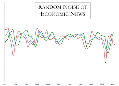
(Economic Data Source: Economic Cycle Research Institute)
Business Activity is never smooth, and investors are continually bombarded with economic noise. How can an investor make sense of this tangled “economic Gordian knot?”
In reality, there is order to the system and the cycle is continually progressing through a set sequence of events or turning points. Chart 2 attempts to bring order to the chaos featured Chart 1 by separating the three indicators and arranging them in their chronological sequence. Each has been plotted in momentum format in order to emphasize its cyclic rhythm.
Chart 2: Real World Business Cycle Sequence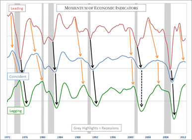
(Economic Data Source: Economic Cycle Research Institute)
Separating the momentum of economic indicators and placing them in sequence brings clarity to the random noise. Business cycle turning points are readily identified, giving investors an important edge.
The names Leading, Coincident and Lagging are derived from the fact that these series are constructed from several economic indicators that lead the economy, coincide with the economy and lag the economy. An example of a leading indicator might be the highly interest sensitive housing market. Nonfarm payrolls, industrial production and Gross Domestic Product (GDP) are examples of coincident indicators. Capital spending tends to increase when factories are humming in the late stages of the cycle and would, alongside the unemployment numbers represent lagging aspects of the economy. Chart 2 clearly demonstrates these indicators live up to expectations as peaks in the leading series form ahead of the coincident indicators, which in turn lead the lagging series. The difference in each cycle lies in the leads and lags as well as magnitude. Cyclical troughs also experience the same chronology.
How do market turning points fit into the cycle?
The lead, coincident and lag sequence is of course a gross over simplification since there are literally hundreds of such turning points for each facet of the economy in any given cycle. The practical benefit of this knowledge is that the turning points of bonds, stocks and commodities are all part of the business cycle sequence. These are shown in Figure 1 together with a theoretical growth path of the economy. In this instance the trajectory is assumed to be that of a coincident indicator such as GDP. Let’s briefly consider how the financial markets fit into the sequence starting with the onset of a recession.
Figure 1: Theoretical Business Cycle Sequence
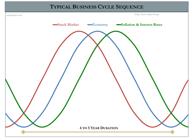
(Source: Pring Turner Capital Group)
The simple bell-shaped curve illustrates continuous change in the economy with one cycle leading into the next. Investors can benefit by observing the normal, sequential, and repetitive nature of the economy.
As Interest rates peak: Own bonds
Most people think that interest rates peak as the economy enters a recession, however the peak typically develops after the recession has already begun. Interest rates are the price of credit and move inversely with bond prices. Like any other item, interest rates are determined by the interaction of supply/demand pressures.
The biggest player on the supply side is the Federal Reserve through its influence on the banking system. One reason why the Fed acts with a lag is because the central bank has to make sure that policy changes are backed up by a solid trend of emerging statistics, which can take some time to develop. When the economy is in full blown growth mode, the Fed is concerned with restraining inflation. However as the economy moves into a recession the Fed comes to the realization that unemployment and not inflation is their main concern and therefore injects liquidity into the system. In the meantime the weakening economy reduces the demand side of the credit picture. Declining demand and increasing supply leads to lower interest rates. As interest rates drop, bond prices rally.
Maximum Economic Pessimism: Stocks Bottom Out
As interest rates peak the seeds are being sewn for the next economic recovery. The stock market is a leading indicator and does not wait for good economic news but instead discounts it ahead of time. In the depths of recession and after interest rates have declined and bond prices appreciated, the stock market begins to turn up. This befuddles most investors because the stock market begins a dynamic cyclical advance when the economic news cannot be any worse. A stock market bottom by definition is the point of maximum pessimism. Knowledgeable investors take advantage of the stock market’s character to be one of the most dependable leading indicators. It still takes courage (and cash) to buy stock in the midst of miserable economic headlines. At this point in the business cycle two asset classes are in cyclical bull market, bonds and stocks, while commodities are still underperforming.
Economic Growth Leads to Higher Commodity Prices
Typically commodity prices continue their bear market until after the economic recovery gets underway. As the economy picks up steam, the demand for raw materials increases. Usually commodity prices do not experience a sustained rally until fundamental demand from real users as opposed to speculators sets in, and this can only happen when the economy has emerged from the recession. At this point in the business cycle all three asset classes are in cyclical bull markets. This is distinctive of this part of the business cycle where all three asset classes are doing well, and everyone is an investment genius.
Interest Rates Bottom and Bond Prices Peak
At this point in the cycle all three markets are in a rising trend, but like all good parties, this one too must come to an end. As signs of a more robust economy appear there is no longer any pressure on the Fed to continue with an easy money policy so they start to turn off the monetary printing presses. The policy does not immediately turn into a tight one, just less accommodative. This shift, along with an increasing demand for loans as consumers and businesses are willing to take on more debt, has the effect of pushing up interest rates, which leads to falling bond prices. Provided profits can rise at a faster rate than interest rates the stock market is able to extend its rally. Not all equity sectors participate though, because rising rates usually have an adverse effect on interest sensitive stocks. Additionally, bond equivalents, such as preferred shares, have to compete with bonds themselves. This means that their yields must rise to meet that competition, and prices must fall accordingly. As a result, while the overall market as reflected in the S&P Composite might extend its bull market, breadth begins to narrow as fewer stocks are now participating in the bull market.
Anticipating the Next Recession: Stocks Peak
Eventually stock market participants sense the trend of rising rates has progressed to the point that a slowdown or actual recession will result. Like anyone standing on a railroad track and knowing a train is coming, stock holders do the logical thing and get off the track right away. Not all stocks move lower as those benefiting from higher commodity prices, such as basic industry, mining and energy experience wider profit margins and usually manage to extend their gains at this point.
The Slowing Economy Push Commodities Lower
Eventually though, strains on the system begin to emerge. The trend of sharply rising commodity prices encourages the Fed to be far more aggressive in its monetary policy, and the Fed begins to tighten. This renewed push on higher rates breaks the back of those sectors of the economy that are still expanding, including the commodity area. Sagging demand for resources resulting from the slowing economy pushes commodities into their cyclical downturn. Commodities peak out, either at the very end of the recovery, or occasionally in the opening moments of the recession. Now all three asset classes (bonds, stocks, and commodities) are declining. The business cycle is complete, and the next step is to anticipate the move to the beginning of the cycle for a repeat of the process.
The Double Cycle
Occasionally the growth path of the economy does not experience an actual contraction but instead bottoms out close to the equilibrium point (0% GDP growth). This phenomenon is known as a growth recession because it is only a “recession” in terms of the growth curve. We call this a double cycle because the rotational bond, stock commodity process develops twice. Growth recessions develop when the recovery is not particularly robust and few distortions are therefore created. This means the self-correcting mechanism of the business cycle has less work to do, so the decline in the growth path is therefore a mild one. Subsequently, the economy gets a second wind and in this second part of the recovery the economy experiences distortions because capacity utilization levels are improving from a higher level. Generally speaking the longer an economy goes without a negative correction the greater the degree of confidence that builds up. There is, of course, nothing wrong with confidence. The problem develops when people become overly confident, because that’s when careless decisions are made. The real estate developer who builds far too many houses, the banker that lends the developer the money to build the homes. The buyer who purchases a bigger house because he extrapolates his recent commission earnings trends in an everlasting linear uptrend and so forth.
Introducing the Six Stages
Like the seasons of the year, the environment for bonds, stocks, and commodities also progress in a repeatable and sequential fashion. Many investors are unaware of and unprepared for the ever-changing financial market seasons. Anyone with gardening experience understands it is difficult to plant in the winter because nothing grows. The same is true for the financial seasons in the business cycle, where investors can use knowledge of the chronological bond, stock, and commodity sequence to create a financial market roadmap. By better understanding these financial seasons and using the correct forecasting tools, investors can make well-informed decisions and dramatically improve their chances for investment success. Each asset class has two turning points in a given business cycle—a top and a bottom. This means that a typical cycle has a total of six junctures—three buys and three sells. We call these the Six Stages.
Figure 2: Pring Turner’s Six Stage Business Cycle Stages
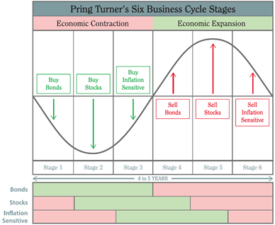
The six-stage model can help investors dynamically adjust asset allocations around the typical business cycle sequence. Essentially an investor needs two game plans one for defense to protect assets in difficult periods and one for offense to grow wealth during favorable conditions.
The stages are illustrated in Figure 2 and begin with bonds in a bottoming mode and continue all the way through until the eventual peak in commodity prices. The implication from the diagram is that each stage is equal in duration, but in reality this is not the case. Occasionally two markets may reverse simultaneously. This is what happened in October 1966 when both bonds and stocks bottomed together. In such a situation the cycle moves from Stage 6, when all three markets are declining, directly to Stage 2, where bonds and stocks are bullish and commodities bearish. Stage 1, in which bonds are bullish and the other two markets are bearish, is therefore bypassed. The sequential approach described here is by no means automatic. If it worked like clockwork in every cycle, everyone would be using this approach and it would be instantly discounted. Our research indicates that the six stages move sequentially approximately 85 percent of the time, which offers an edge for investors.
How do we know which stage we are in?
The stages are identified through models or “barometers” for each of the three asset classes. They are constructed from technical, economic and inter-market relationships that have been researched back to 1955. Charts 3 thru 5 demonstrate their performance. The status of each barometer is used to identify the prevailing stage of the cycle. Stage I occurs when bonds are positive and stocks/commodities are negative. Stage II occurs when bonds and stocks are positive while commodities remain negative; as so on and so forth. At Pring Turner we use this stage information to establish the basic tactical asset allocations guidelines for our investment portfolios.
The green and red bands in the bottom of Figure 2 show when each asset class is positive (green) or negative (red). For example bonds are positive in stages 1 thru 3, stocks in stages 2 thru 4 and commodities stages 3 thru 5.
Chart 3: Pring Turner Bond Barometer 1956-2012
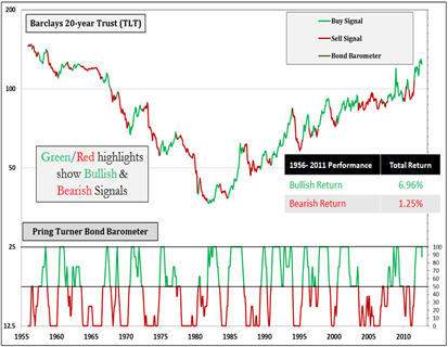
Chart 4: Pring Turner Stock Barometer 1956-2012
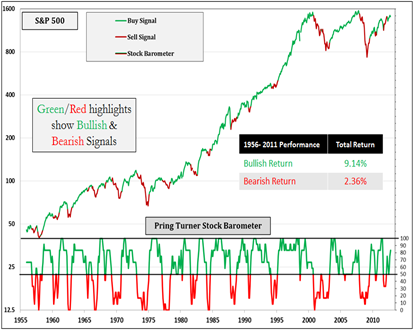
Chart 5: Pring Turner Inflation Barometer 1956-2012
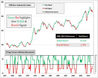
The barometers define favorable or unfavorable environments for bonds, stocks, and commodities, when combined together the barometers define the business cycle stage.
Applying business-cycle stage shifts to tactical asset allocation changes
The key point in applying stage shifts to changes in tactical asset allocation is viewing asset allocation within the context of understanding the risk and reward characteristics of the different asset classes at each stage of the economic cycle.
Table 1: Broad Business Cycle Asset Allocation Guidelines
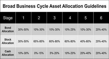
This broad asset allocation guideline can serve as an important starting point for actively managing portfolios throughout the business cycle.
For instance, during a recession in Stage 1 the allocation includes a healthy mix of bonds and cash to stabilize portfolio values. The opposite is true in Stage 3, when the economy is running at full throttle and maximum exposure to stocks is recommended. We believe that our six-stage framework is an ideal way to construct an active allocation discipline, especially because it also serves as a critical risk-management tool. Keep in mind that no strategy or discipline is perfect and that each has its own shortcomings. In the case of economic fluctuations, not all cycles will experience every stage, and stages occasionally diverge from the expected sequential order. Sometimes the cycle will skip a stage or even two. In fact a cycle may also retrograde to a previous phase. These are additional reasons why changes to portfolio allocations should be gradual. Larger allocation switches can be justified only when the evidence of a change in the environment is overwhelming and markets have not already gone too far in factoring this into prices. For investors, the beauty of following the repetitious nature of the business cycle is an investment methodology that never goes out of style, an “all season” approach if you will.
Does this business cycle stuff really work?
It is certainly a reasonable question to ask whether this approach has actually worked in the real world. In 2012 S&P Dow Jones Indexes in conjunction with Pring Research launched the Dow Jones Pring Business Cycle Index. The Index itself incorporates a rules based system to identify the six stages and optimizes asset allocation in conjunction with sector rotation according to how each asset class and sector has traditionally performed in that phase of the cycle. The performance of the Index by stage is shown in Table 2. The two starting dates differ because the ETF instruments or tracking indexes used in the Index were not available prior to 1994 so proxies were used between 1955-1994.
Table 2: Dow Jones Pring Business Cycle Index Performance by Stage 1955-2011 and 1994-2011
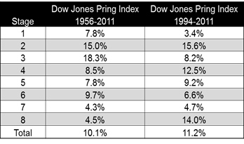
(Source: Dow Jones Indexes)
The combination of tactical asset allocation changes and effective sector rotation throughout the business cycle resulted in positive returns in every stage (on average) and impressive risk-adjusted returns. Note: Some individual stages experienced negative returns and future results will vary.
What the Dow Jones Pring Index illustrates is the combination of tactical asset allocation changes and effective sector rotation throughout the business cycle resulted in positive returns in every stage (on average) and strong risk adjusted returns during the 1956-2011 & 1994-2011 timeframes. Not every stage in every cycle experienced positive returns but over the long-term the real world approach supports the theory.
Dow Jones Indexes put together a nice performance illustration (Chart 6) which compares the performance of the Dow Jones Pring Index with the three main asset classes over the 1956-2011 investment horizon.
Chart 6: Dow Jones Pring Business Cycle Index Performance 1955-2011
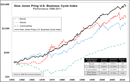
Since 1956, the Dow Jones Pring U.S. Business Cycle Index has outperformed all three asset classes while experience roughly two-thirds the risk (volatility) of the U.S. stock market. (Source: S&P Dow Jones Indexes).
The table within chart 6 compares the return performance of the Index with the three asset classes in addition to a comparison of risk using (standard deviation, volatility) calculations. It shows that not only did the Index outperform the S&P but did so with lower risk (standard deviation, volatility).
Summary
- Markets have tracked business cycle sequences for over 150 years – since the industrialization of the U.S. economy.
- Financial markets are linked rationally, logically, and sequentially to the business cycle which are driven primarily by human psychology.
- Paying attention to the normal swings in the economy is an enormous help to investors.
- Pring Turner organizes the business cycle into six stages to identify which asset class and sectors to favor or underweight in each stage.
- The stages are identified with the use of Pring Turner’s proprietary “barometers” for bonds, stocks, and commodities.
- Optimal asset allocation and sector rotation for portfolios can be adjusted based on the business cycle stage in an effort to increase returns while reducing risks.
© AdvisorShares