The standard 60/40 portfolio featuring a basic mix of US and international equities plus aggregate bonds has returned a cumulative 754% since 1990. Or has it returned 781%? Or maybe 730%?
All three numbers are correct for this standard strategic asset allocation mix. The differences, however, like the devil, are in the details: it depends on when the portfolio was rebalanced.
Think about portfolio rebalancing like Marty McFly purchasing the Grays Sports Almanac when he and Doc Brown traveled to the year 2015, only to have it found by the 2015-version of Biff Tanner after Doc Brown haphazardly threw it out. This led the 2015 Biff to travel back to 1955 to give it to his younger self so he could get rich by betting on sporting events. In essence, this one singular action triggered a chain reaction of events, thereby creating a distorted time paradox and an alternate timeline for everyone involved.
That’s the impact of rebalancing. The players remain the same, but the timeline has been altered. And depending on the frequency, the difference between the returns could be as stark as the difference between the idyllic original Hill Valley in 1985 and the dystopian “Hell Valley” 1985A version.
Splintered return streams due to rebalancing have been well documented in some respects. The turn of the month effect1 has often been showcased, as has the notion of timing luck2and how it can manifest in different return patterns. Yet in my travels and conversations with investors, it rarely comes up—even though this is an aspect investors should be acutely aware of, particularly during the strategy due diligence and performance attribution process.
To demonstrate how disparate the return patterns can be, I ran a few simulations on the standard 60/40 portfolio dating back to 1990. The analysis shows that there’s no perfect rebalancing period and the decision to rebalance can create yearly return patterns that can at times differ by more than 8%. Imagine losing out to a competing standard strategic model by 8% in a given year just because the portfolio was rebalanced quarterly instead of annually.
Is there a 1.21 gigawatts frequency for portfolio rebalancing?
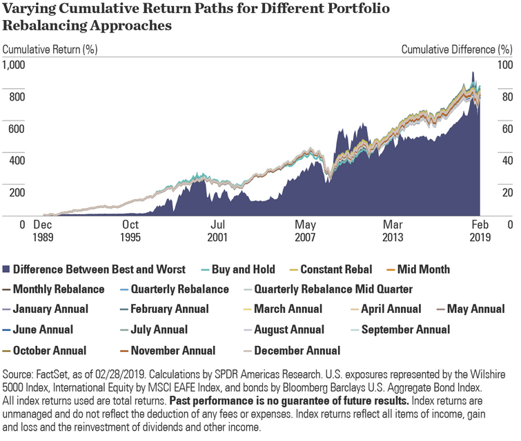
The below chart shows the cumulative returns of the 60/40 portfolio rebalanced at different intervals (e.g., monthly, quarterly, semi-annually, annually), as well as a portfolio rebalanced annually but at differing times (e.g., March, May, July). The difference between the best and worst portfolios on a cumulative basis compounds over time, standing at 81% currently. What’s more interesting is that the leading portfolio with the best cumulative return changes frequently, telling us that there’s no perfect frequency—unlike the amount of electricity (1.21 gigawatts) the flux capacitor in the DeLorean needs for time travel.

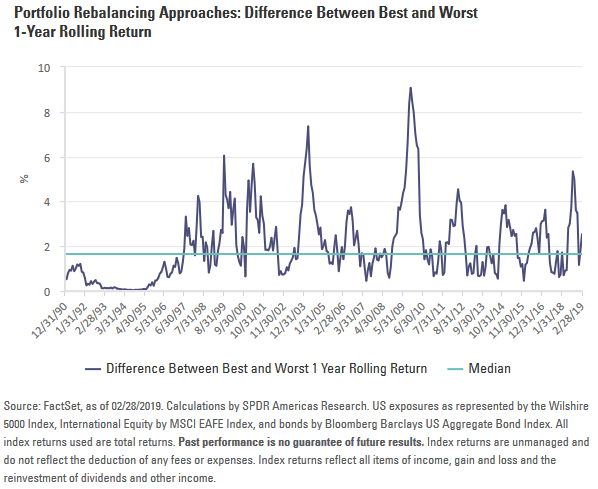
While leadership changes and cumulative returns are different, the above chart doesn’t show the variability of inter-period returns that can result from rebalancing the same assets at different times—particularly around volatility events. As shown below, rolling 1-year returns demonstrate how differentiated the return paths can be—much like how the ripple effect of one event can cause the historical Hill Valley Court House to become the site of the Biff Tanner Pleasure Paradise Casino & Hotel.
Great Scott, this rebalancing stuff is heavy
Once a path is altered, there’s no going back to the original. This was even true for Marty and Doc, who had the opportunity to go to 1985 and correct the altered timeline, but in doing so they created a 1985B timeline. The same is the case for portfolio rebalancing: Once a period is selected, the return path has been splintered.
So what should investors do about it?
There are many options to counterbalance, though not solve, the randomness of rebalancing:
- Create overlapping portfolios that are rebalanced at different times (i.e., tranching);
- Target rebalancing to fixed percentage weights based on bands (e.g., equities can’t be more than 65%); or
- Select a period based on striking a balance between exposure management and costs, as more frequent rebalancing will increase turnover and transaction costs.
The latter approach accepts the reality that there’s potential for either a world where Biff Tanner owns a casino or one where he owns an auto detail shop. This approach embraces the randomness of inter-period returns, and takes a longer-term view that the short-term deviations have the potential to even out given the frequent changes in leadership. It requires the investor to justify the rebalance period as a simplistic calendar approach seeking to provide consistent asset class weights while mitigating transaction costs in managing to a strategic benchmark.
Given the difference in returns between rebalancing schemes, taking this view on a short-to-intermediate term basis would indeed be a leap of faith for investors—similar to viewers ignoring one of the biggest plot holes in the Back to the Future franchise: that Marty’s parents wouldn’t recognize him when he got older (e.g., in 1985) as looking just like the person in 1955 (when Marty was pretending to be Calvin Klein) who introduced them and started their romance.
No matter the method chosen to rebalance portfolios, the frequency selection should always be emphasized during the due diligence and performance attribution process for any given strategy. Investors should expect to be provided with a rationale as to why the defined course of rebalancing action was taken.
For more insights on portfolio construction, check out our new Spotlight On series that looks at efficient asset allocation and the many sub-asset classes that can comprise a diversified portfolio.
© State Street Global Advisors
Read more commentaries by State Street Global Advisors