Putting ‘Fixed Income’ Back Into Fixed Income: Cash-Flow-Matched Bond Strategies for Retirees

Despite this historically bad year for bond returns, not a single investment-grade corporate bond defaulted in 2022.² Anyone who was holding those bonds to maturity and collecting the cash flows – rather than being forced to sell them to raise cash – had a totally normal, boring, and expected year in their bond portfolios. Every dollar of promised cash flow was paid.

As many advisors know, bond math is notoriously counterintuitive. When interest rates rise, as they did in 2022, the price of fixed-coupon bonds fall. So, if you had to sell part of your client’s portfolio to generate cash flows, 2022 would have hurt quite a bit. Your bond portfolio would not have felt much like “fixed income.”

In contrast, when bond prices fall, nothing at all happens to the coupons and principal payments of fixed-coupon bonds. Those cash flows are promised in the bond indenture, a legal contract between the issuer of the bond and the bondholders. For example, if a corporation issues a 5% coupon bond and they hold up their end of the contract (i.e., the bond does not default; defaulting is often synonymous with bankruptcy), the bond will pay out its 5% coupon per year and principal at maturity regardless of what happens to the price of the bond.

Cash flow matching

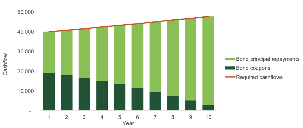
Investors in need of cash flow, like retirees, can take advantage of the contractual nature of bond coupons and principal repayments by creating a cash-flow-matched bond strategy. In this strategy, bonds are selected such that the coupon and principal repayments from the bonds add up to the cash flow needs of the client.

Unlike a traditional rolling bond ladder, in which proceeds from bonds are reinvested, a cash-flow-matched bond ladder is largely immune from interest rate risk. Once purchased, the targeted cash flows will be paid, regardless of what happens to interest rates – as long as the bonds do not default. And with sufficient diversification across bond issuers, default risk decreases.

If you tried to generate the same cash flow with a traditional constant-duration bond portfolio (like most bond funds and ETFs), you add two significant risks: 1) you will be forced to sell at a loss when rates are high (and bond prices are low); and 2) you will have to reinvest when rates are low (and bond prices are high). Cash-flow-matched bond strategies use the same universe of bonds, with the same yields, but they are engineered in a way that protects investors from these risks.

Why aren’t more advisors using this strategy?

There are likely many reasons so few advisors use cash-flow-matched bond strategies, but one we hear often is this approach must be suboptimal from a total return perspective: If you optimize a portfolio for total return relative to risk, any deviation from that portfolio means it is suboptimal. Additionally, the idea that you’d purposefully consume principal early in retirement is counterintuitive, compared to an optimized total return portfolio that seeks to grow or preserve principal over time.

There are two flaws with this way of thinking.

First, typical portfolio optimization does not account for cash flows; it’s just trying to maximize risk-adjusted return over the long run. If we account for cash flows, adding a cash-flow-matching strategy to a total return portfolio appears to improve risk-adjusted returns.

Second, there is reason to be suspicious of the assumptions involved in total return investing. Cash-flow-matching strategies require fewer assumptions, giving retired clients greater certainty of getting the cash flows they need.

Together, this means cash-flow-matched bond strategies have the potential to provide both a higher certainty of cash flows and better risk-adjusted total returns.

Cash-flow-matched bond strategies appear to improve risk-adjusted return

Standard portfolio optimization techniques do not account for cash flows.

The common practice we hear from advisors is the following: First, optimize a portfolio for total return relative to volatility, and then run Monte Carlo to simulate the results of withdrawing cash from the portfolio over time. The optimization knows nothing about the cash flows, so it isn’t necessarily optimal given the client’s cash flow need.

Let’s look at an example.

Suppose a client has $1 million at retirement. Their advisor optimizes for total return relative to volatility, given a risk tolerance. Let’s say, simplistically, the optimization lands on the typical 60/40 stock/bond portfolio for a client. The advisor then runs some Monte Carlo analysis in a planning tool to determine that something like the 4% rule works pretty well: The client can take $40,000 each year, adjusted for assumed inflation of, say, 2%.

Alternatively, the advisor could use a cash-flow-matched bond strategy. For example, an advisor might secure the first 10 years of the required cash flows using a cash-flow-matched portfolio of investment-grade bonds. This would consume about one-third of the $1 million over 10 years. With the remaining two-thirds of the assets, the advisor could invest in the same 60/40 portfolio from the total return approach, without having to draw down any cash flows from this part of the portfolio. (See the Appendix for variations on this analysis, showing it is not driven by allocation differences.)

Here’s how the $1 million portfolio value looks after 10 years, based on 1,000 simulations:

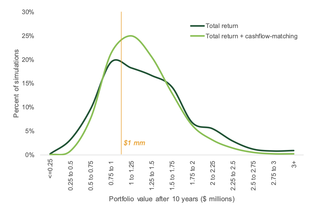
The cash-flow-matching strategy trims the tails of the 10-year outcome for the retiree. It makes it more likely that, after 10 years, the portfolio will be in the $1 million to $1.75 million range than the total return portfolio alone – a solid outcome, given that you’re also generating $40,000-plus per year in cash flow along the way.

Cash-flow-matching also lowers the chance of the worst outcomes happening: The client is less likely to end up with a lot less than what they started with (or to have to reduce spending along the way). This is because cash-flow matching helps protect the portfolio from sequence-of-return risk.

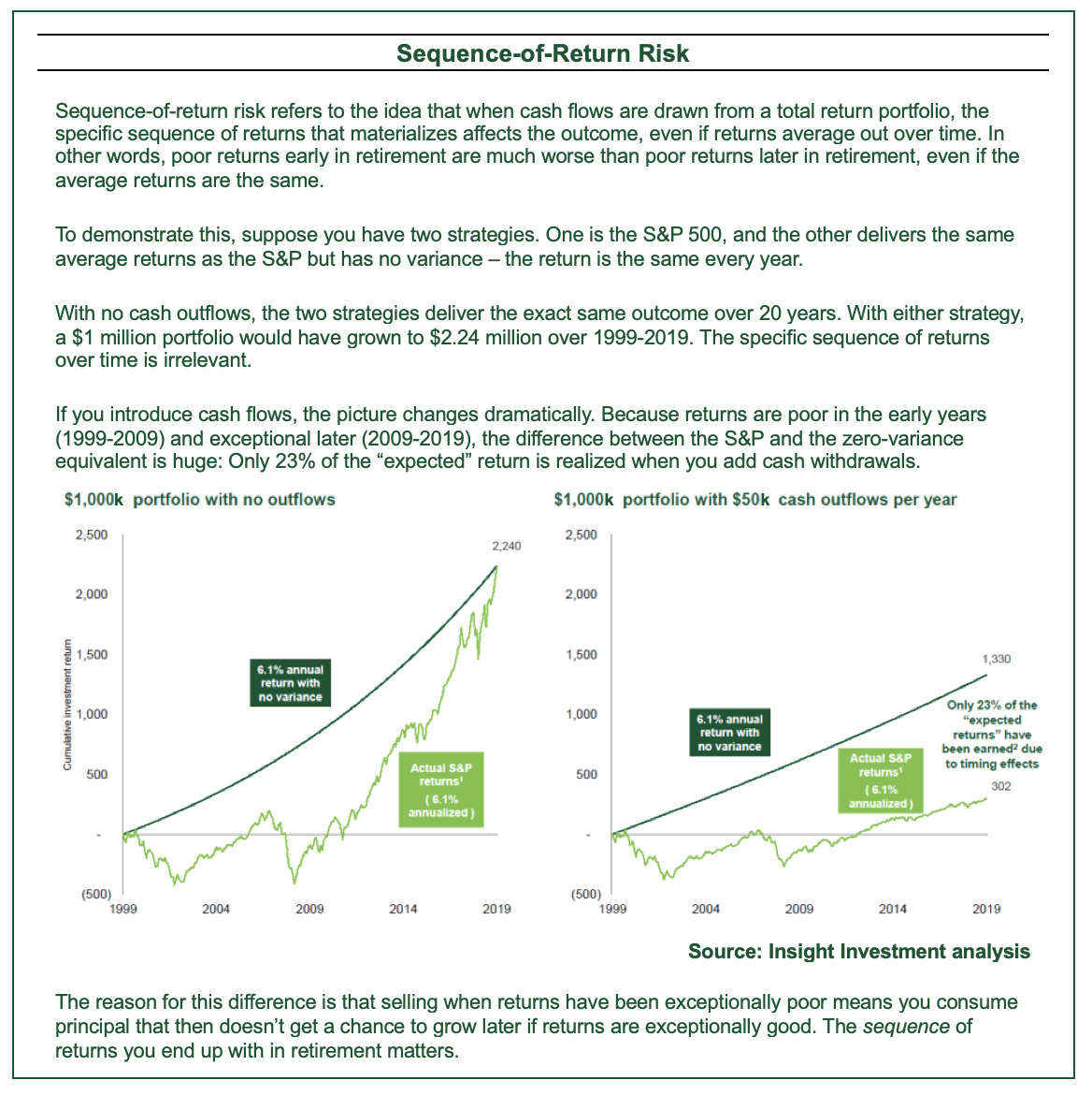
The reason for this difference is that selling when returns have been exceptionally poor means you consume principal that then doesn’t get a chance to grow later if returns are exceptionally good. So even if your capital market assumptions are accurate, the unpredictable sequence of returns you end up with in retirement impacts how much principal you end up consuming. In contrast, cash flow matching gives you predictability of principal consumption for a period of time, allowing the rest of the portfolio to avoid sequence-of-return risk.

The downside of cash flow matching, given these assumptions, is that the portfolio is also somewhat less likely to double or triple in 10 years. But that’s a relatively remote possibility even without cash flow matching, given the return assumptions³ and the fact that the portfolio is paying out cash flows along the way.

Another way to evaluate this strategy is to compare the annualized returns over 10 years. You can see that the distribution of returns gets tighter when we add cash flow matching.

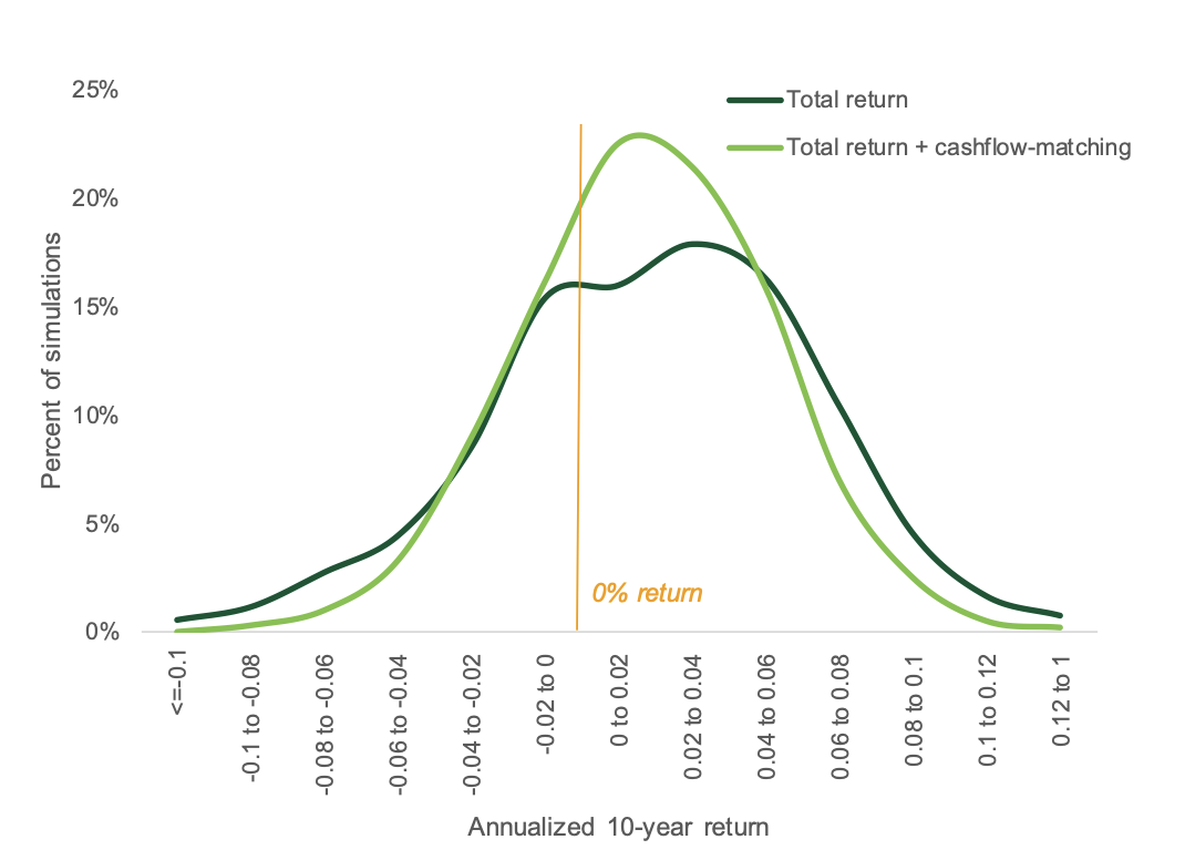
As we saw before, the client is less likely to experience “bad” outcomes (significantly negative returns), more likely to experience “pretty good” returns (despite drawing down), and also less likely to experience “amazing” outcomes. Note that returns here are calculated by comparing the $1 million starting value to the value of the portfolio after 10 years, and then annualizing. In each case, the $40,000-plus of cash flow is being consumed by the client.

We can calculate a simple risk/return ratio to get an idea of whether the reduced likelihood of very high returns is worth the reduced risk of poor returns. The total return approach gives a risk/return ratio of 0.45, meaning the average annualized returns are about half the variability of those annualized returns. The cash-flow-matching risk/return ratio is 0.53, meaning more return per unit of risk.

Making fewer assumptions means greater certainty for your clients

To state the obvious, total-return investing requires assumptions about future returns. But those assumptions are tenuous, and even small errors can lead to big differences in outcomes for retirees. It’s just not easy to predict what will happen to stock or bond prices over time. And if the predictions are wrong, retirees could suffer.

In contrast, the assumptions required for cash flow matching are fewer. If you’re cash flow matching with TIPS or Treasuries, all you need to assume is that the U.S. government will not default. You don’t need a crystal ball to predict future bond returns, stock returns, interest rates, or Fed policy. You just need to know a present value – the current yields of the bonds, which dictate how much investment will be required to secure a given stream of cash flows.

If you’re cash flow matching with municipal bonds or corporates, there is greater default risk. But investing in bonds within a total return strategy requires the same default assumptions; it just also requires assumptions on top of that about future interest rates and spreads.

The effect of fewer assumptions is greater certainty. If you’re making fewer assumptions, that means you’re less likely to be wrong.

And it’s an easier story to tell clients, too. In total-return investing, no one is really on the hook for the cash flows from a portfolio, because whether clients get the cash flows they want, or something different, depends on the accuracy of the total return assumptions and the robustness of the complex modelling techniques (both of which are likely buried somewhere in your planning software).

In cash-flow-matching strategies, someone is very much on the hook: the issuers of the bonds – whether it’s the U.S. government, a local municipality, or a multinational corporation (maybe even the same multinational corporation your clients used to rely on for their salaries). Fixed-coupon bonds held to maturity are contractual promises to pay.

Cash-flow-matched bond strategies deserve consideration for any client in need of cash flow. This approach not only provides greater certainty, it may also be more “optimal” than you think.

Massimo Young, CFA is head of investment solutions and technology for the individual retirement solutions group at Insight Investment.

ENDNOTES

¹ Bloomberg US Corporate Total Return Value Unhedged USD (LUACTRUU) returns for 2022, as of 1/7/2025

² At least according to S&P ratings.

³ See appendix for the assumptions used in the Monte Carlo simulations.

Appendix: Methodology

One potential challenge to the analysis presented above is that the results could be driven by differences in asset allocation rather than the cash-flow-matched bond strategy. However, that is not the case.

Below are two variations of the analysis to show that the specific allocations do not impact the high-level result.

In the first variation, assume the total return portfolio is 100% fixed income. The total-return approach and the total return + cash flow matching are always invested 100% in bonds. The only difference is how those assets are used. In the cash-flow-matched bond strategy, 10 years of cash flows are matched. The rest of the portfolio is invested in a total-return fixed income strategy.

The results are broadly similar to the analysis presented above. Cash flow matching tightens the distribution of returns, reducing the likelihood of poor outcomes, and produces a distribution of 10-year annualized returns with a better risk/return ratio.

100% bonds: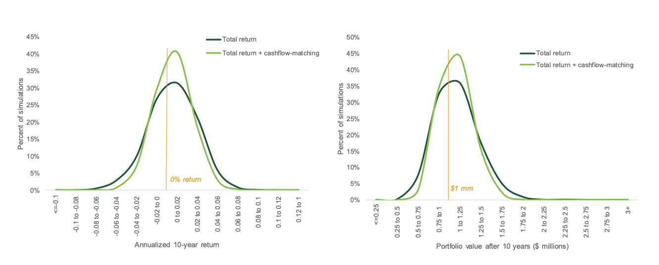

The other variation is at the other end of the spectrum: 100% stocks for the total-return portfolio. This allocation also produces a similar result in that the cash flow matching “trims the tails” of the distribution:

100% stocks: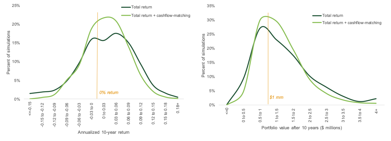

Appendix: Assumptions

• 60/40 portfolio: All assumptions use a 10-year horizon from 2024 Horizon Actuarial Survey of Capital Market Assumptions
  • Stocks:
    • U.S. Equity: Large Cap
    • Forecasted arithmetic return: 7.74%
    • Forecasted standard deviation: 16.52%
  • Bonds:
    • U.S. Corporate Bonds: Core
    • Forecasted arithmetic return: 5.10 %
    • Forecasted standard deviation: 5.90%
  • Correlation: 0.28
• Cash-flow-matched portfolio:
  • IRR of 5.10%, same as Corporate Bond assumption in total return portfolio
  • Assume perfect cash flow matching and no defaults
  • Sense-check on yield assumption:
    • Based on the Treasury spot curve as of 1/7/2025, the IRR of a cash-flow-matched portfolio targeting a 10-year cash flow with 2% COLA is 4.6%
    • Using BVAL or BAML spread curves on top of that, a portfolio of Corporates rated A would have an IRR of 5.2%-5.3%
    • Therefore, an IRR of 5.1% is a reasonable assumption for an investment-grade portfolio with low default risk (i.e., between credit rated A and AA)

A message from Advisor Perspectives and VettaFi: To learn more about this and other topics, check out some of our webcasts.

Read more articles by Massimo Young