In our last post, we covered the importance of a well-designed investment universe as a precondition for thoughtful diversification. In this second article on Dynamic Asset Allocation for Practitioners, we will explore several methods for measuring price momentum to compare and contrast their utility under different portfolio concentration and asset universe specifications.
What is momentum?
Momentum is the tendency for an asset’s price to continue in its current direction. There have been countless studies of this effect in virtually every market around the ranging from vanilla stocks and bonds to real estate and fine art (and everything in between). Furthermore, research shows the momentum effect has existed since at least the thirteenth century.
Academics have presented myriad explanations for why this phenomenon is so universal, but our preferred explanation involves human behavior. Specifically, in uncertain situations, humans quite logically take cues from each other about how they should act. Agent models of this behavior always manifest in informational cascades that, when applied to capital markets, may create momentum effects.
The identification of human behavior as the driving force behind momentum is strengthened by prospect theory, which states that investors feel the pain of realized losses far more acutely than joy of realized gains. As a corollary, investors tend to hold depreciating assets to avoid the pain of realized loss, while quickly selling appreciating assets to lock in small wins. This dissonant trading behavior creates downward pressure on appreciating assets, causing them to take longer to achieve their fair value. Of course, it also creates an opportunity for momentum investors to harvest the gains left unclaimed by the herd.
These deeply-engrained behavioral shortcomings make momentum a “premiere anomaly” that expresses useful and actionable signals.
The balance of this series will present ways to harness the momentum effect across global asset classes. The strategies we present will be long-only because such approaches harness two major sources of return: the long-term premia derived from exposure to risky assets (as opposed to cash), and the multi-asset momentum factor itself. In later articles, we will demonstrate that about half the performance of Adaptive Asset Allocation strategies are derived from consistent exposure to long-only global risk premia, with the balance attributable to active momentum bets.
Overfitting via Investment Universe, Concentration, and Rebalancing Frequency
To revisit the main themes from Part 1, recall that our investment universe is composed of the following 12 global asset classes representing all major asset categories and economic regions of the world. Our goal is to capture the major muscle movements of the global economy, and monetary dynamics.
- Commodities (DB Liquid Commodities Index)
- Gold Bullion
- U.S. Stocks (S&P 500)
- European Stocks (FTSE Europe Index)
- Asia Pacific Stocks (MSCI Asia Pacific)
- Emerging Market Stocks (FTSE EM)
- Global REITs (Dow Jones Global REITs Index)
- Intermediate Treasuries (Barclays 7-10 Year Treasury Index)
- Long Treasuries (Barclays 20+ Year Treasury Index)
- Intermediate International Government Bonds (Unhedged)
- USD Denominated Emerging Market Bonds
- Long-Term TIPs
The investment universe can itself serve as a source of “curve fitting,” as it is easy (not to mention tempting) to alter the universe of potential investments for the purpose of improving simulation results. For example, if one or two assets happen to have done particularly well over our test horizon (U.S. equities, anyone?), or happen to have been particular “trendy.” a simulation’s success may be more attributable to a lucky investment universe than robust selection methods. And finally, holding periods may introduce both frequency and “trading day” biases.
To mitigate these risks, we will run backtests with the following safeguards:
- Simulations will be run on all combinations of 10 and 11 assets drawn from the 12-asset universe.
- Simulations will test concentrations of top 2, 3, 4 and 5 assets.
- Simulations will use weekly, bi-weekly, tri-weekly and monthly rebalancing.
- For weekly rebalancing, we will test trading on each day of the week. For bi-weekly, we run tests that trade on each of the 10 days, etc. As such, we eliminate all day-of-the-month effects, and concentrate exclusively on the momentum signal (and eventually the portfolio formation method as well).
In this way, we will have 79 universes, four levels of portfolio concentration, and 51 day-of-the-month / holding periods. For robust validation, each price momentum methodology will have to show promise across a broad set of these 79*4*51 = 16,116 simulations.
First, our Conclusion: In General, Momentum Works
Momentum is a powerful tool for asset allocation. However, while we can confidently eliminate some methods as being significantly worse than others, those that remain tend to have statistically indistinguishable differences in performance. As a result, the best approach is probably to combine the better performing methods together into one meta-strategy. There is no way, in practice, to be specifically correct by choosing a single approach.
But as with all investing, the goal should be to be generally correct, and to avoid being specifically wrong.
Defining Our Momentum Metrics
Momentum can be defined in myriad ways. We have selected eight different price momentum indicators; the intuition being that they capture a broad spectrum of the more popular methods. Our purpose for investigating momentum is not to “beat the market,” but rather to stabilize a portfolio’s performance across economic regimes, and enhance risk-adjusted returns. We are seeking consistent growth potential in order to allocate capital efficiently and routinely in all market conditions.
The following is a breakdown of each of the momentum indicators tested. To avoid any confusion, we use the same notation for each:
-
n – The “lookback” parameter. Simply the number of trading days we are observing to make our measurement.
-
t – The current price or period.
Metric 1: Total Return (ROC)
The most common measure of momentum strength, where assets are ranked by their rate of change (percentage return) over n days.
![\[T.R.Momentum=\frac{AdjPrice_t}{AdjPrice_{t-n}}-1\]](data:image/gif;base64,R0lGODlhAQABAIAAAP///wAAACH5BAEAAAAALAAAAAABAAEAAAICRAEAOw==)
Metric 2: SMA Differential
This is the rate of change between two different simple moving averages where the lookback period, n, of our numerator is 1/10th the lookback period of our denominator. So, if we are testing the 20-day lookback period, our metric will be the rate of change between the 2-day simple moving average and the 20-day simple moving average.
Metric 3: Price to SMA Differential
Similar to the SMA Differential except that we will use today’s price in the numerator instead of a shorter simple moving average. This gives us a measure of our current price relative to its n-day simple moving average.
Metric 4: Instantaneous Slope
Here we will measure the rate of change between today’s n-day simple moving average and yesterday’s n-day simple moving average.
Relative Time-Series Momentum
The next three metrics compare the current price of an asset relative to the distribution of that asset’s prices over the recent past.
Metric 5: Price Percent Rank
The idea is that we’re forming a distribution of our prices over n days and giving the current price a ranked value between 1 and 100 relative to its own price distribution. This is a non-parametric ranking method, with the formula
Metric 6: Z Score
For those unfamiliar with statistics, a Z score is a way of normalizing a distribution of numbers around a mean (average) based on how far that number deviates from the mean, in units of standard deviation. Scores may be negative or positive and typically range from 0 to ±3.
Metric 7: Z Distribution
This method transforms our Z score into a percentile value bounded between 0 and 1 based on the Normal distribution. Here we are making a key assumption: If you took a sample of prices from any individual asset in our universe and calculated its mean (average); then took another independent sample and calculated its mean; and then kept repeating this process to infinity; the distribution of these means would precisely fit a bell curve. We’re using this transformation as a way to determine the strength of the trend as the price accelerates away from its mean. For those following in Excel, the command for this transformation is Norm.S.Dist(Z score, TRUE).
Metric 8: T Distribution
Here we will be transforming a t-score into a percentile rank using the Student’s t-distribution and a degree of freedom (n – 1). The main differences, between this and the Z-score transformation are based around some of our underlying assumptions; t-scores may more adequately represent our distribution when the sample size is small.
Now that we are collecting momentum scores across several lookbacks. We must then aggregate the scores in a way that makes sense. We cannot simply average an instrument’s scores together due to the high variance between the shorter end of the lookback horizons and the longer end. Rather, we will compare the momentum scores across asset classes independently at each lookback. We will then calculate each asset’s contribution to the total aggregate momentum measured across all assets, by dividing each instrument’s score by the sum of the absolute values of all the scores in the group. These scores are then averaged across each lookback to arrive at a final score for each asset.
Analysis of Performance Distributions
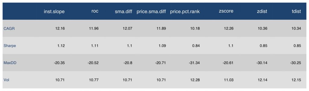
The following table describes the median result for each strategy, simulated from 1991 through March 2017, on daily total return data across all simulation variations.
Figure 1: Median Performance by Momentum Methodology
Source: Global Financial Data, CSI Data, ReSolve Asset Management
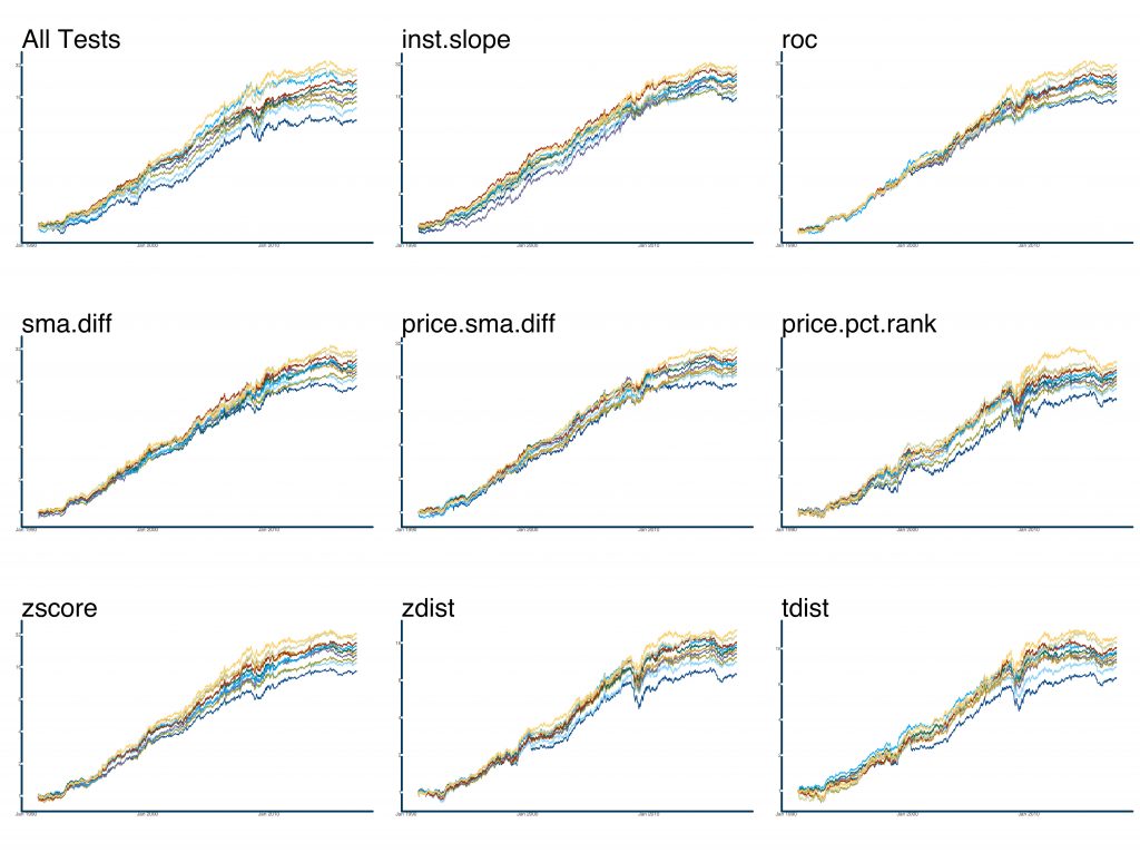
Of course, the median is only one way to gauge performance. Let’s examine the total range of outcomes from all 128,928 tests. The following charts show the simulation results for each strategy at each decile of terminal wealth. Pay special attention to the visual dispersion of results across the deciles, as this provides a clue about the stability of the method.
Figures 2 – 10. Decile Equity Lines of Momentum Methods
Source: Global Financial Data, CSI Data, ReSolve Asset Management
As we can see from these charts there is a large dispersion of performances with peaks and valleys occurring at different times, although all show large declines during 2008. Visually, it’s clear that instantaneous slope provides the tightest distribution of results, suggesting it may provide the most robust signal overall, though ROC, SMA Differential, and Price-SMA Differential all look relatively stable. The Z-Distribution and t-Distribution methods, along with Price Percentile Rank, show a combination of weak overall performance and large dispersion, suggesting they may be particularly unattractive methods.
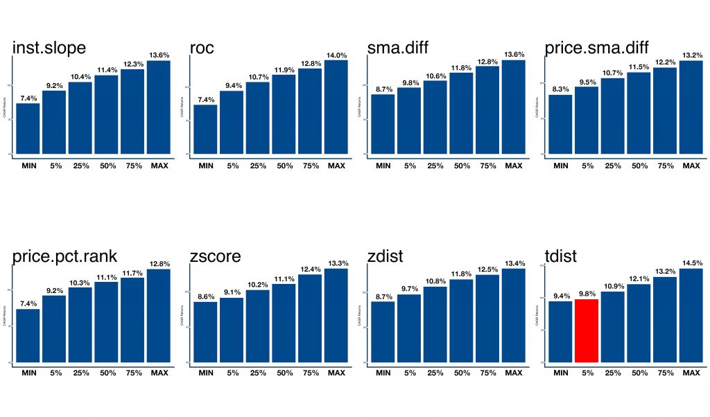
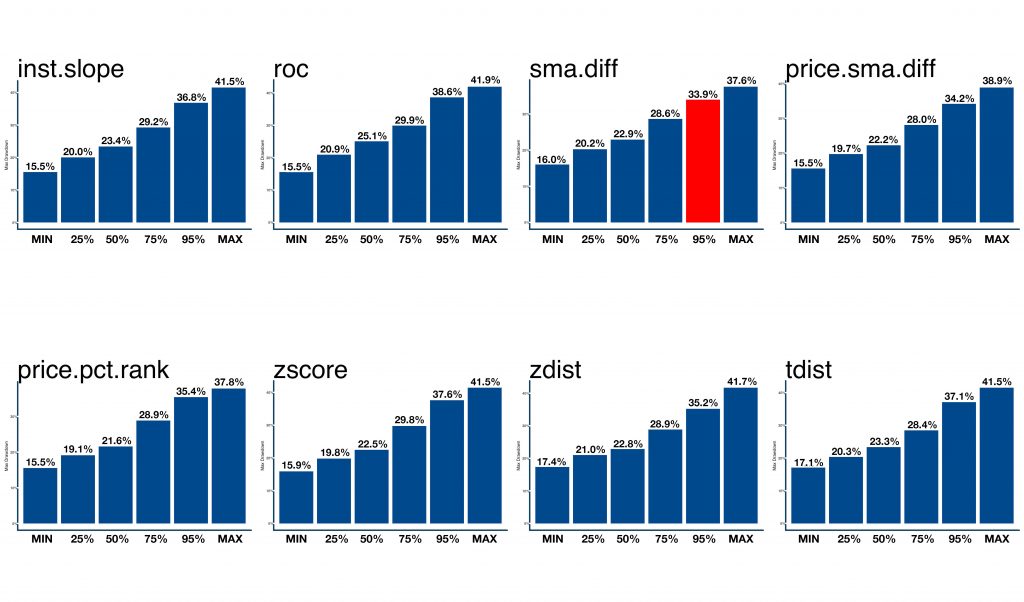
The following charts are cumulative quantile plots of the performance statistics across all combinations of each momentum system. In our opinion, the most realistic way to evaluate the performance of a system is at the most punitive end of the distribution. In other words, we want to focus on methods that perform the best when they are at their worst. As traditional tests for statistical significance focus on the 5th percentile of outcomes, we have highlighted the strategies with the best results at that level.
Figures 11 – 18. Compound Annual Growth Rate by Quantile
Source: Global Financial Data, CSI Data, ReSolve Asset Management
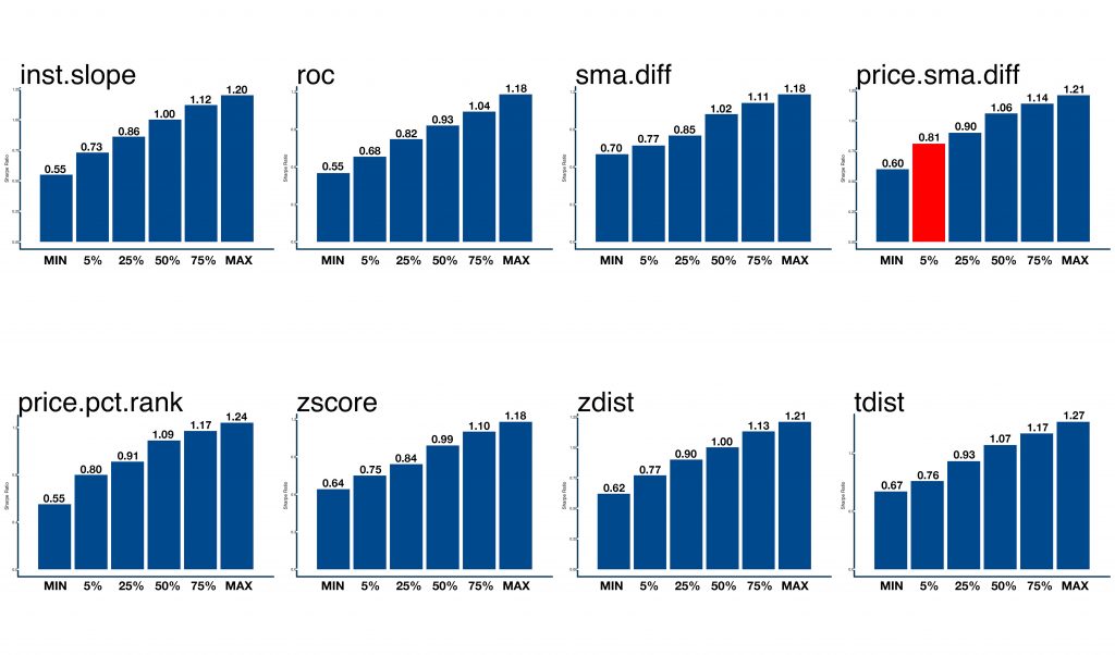
Figures 19 – 26. Sharpe Ratio by Quantile
Source: Global Financial Data, CSI Data, ReSolve Asset Management
Figures 27 – 34. Maximum Drawdown by Quantile
Source: Global Financial Data, CSI Data, ReSolve Asset Management
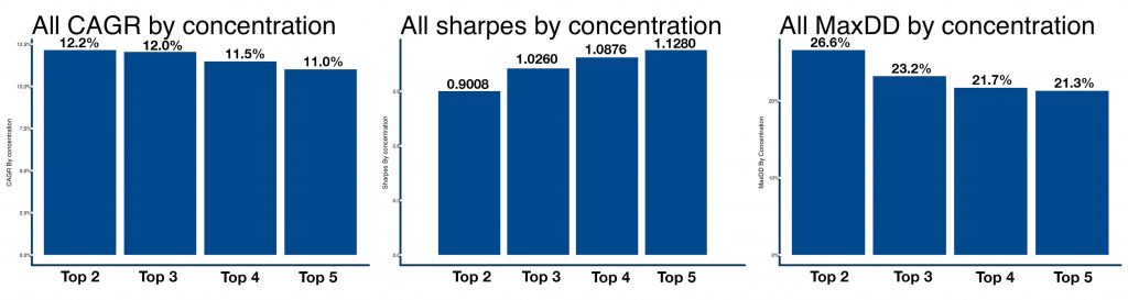
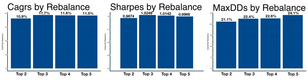
It is also useful to observe the distribution of results for different levels of portfolio concentration, and different rebalance frequencies/holding periods. The following charts break down the average compound returns (CAGR), Sharpe ratios, and maximum drawdowns across momentum methods, along each of these dimensions. The distribution of statistics turns out to be quite intuitive: While the rebalancing periods appear to have little overall effect (except perhaps in terms of drawdown), the highest average CAGRs belong to the most concentrated portfolios, while more diversified portfolios offer lower drawdowns.
Importantly, based on Sharpe ratio, investors embracing diversification gain far more in risk management than they give up in performance. And despite the reality that you “can’t eat Sharpe ratio,” investors are far better served leveraging diversified portfolios than they are concentrating their portfolios to achieve required returns. We will discuss this at length in future articles.
Figures 35-37. Average CAGR, Sharpe, and Max Drawdown Across Holding Concentrations
Source: Global Financial Data, CSI Data, ReSolve Asset Management
Figures 38-40. Average CAGR, Sharpe, and Max Drawdown Across Rebalancing Periods
Source: Global Financial Data, CSI Data, ReSolve Asset Management
INDICATOR DIVERSIFICATION
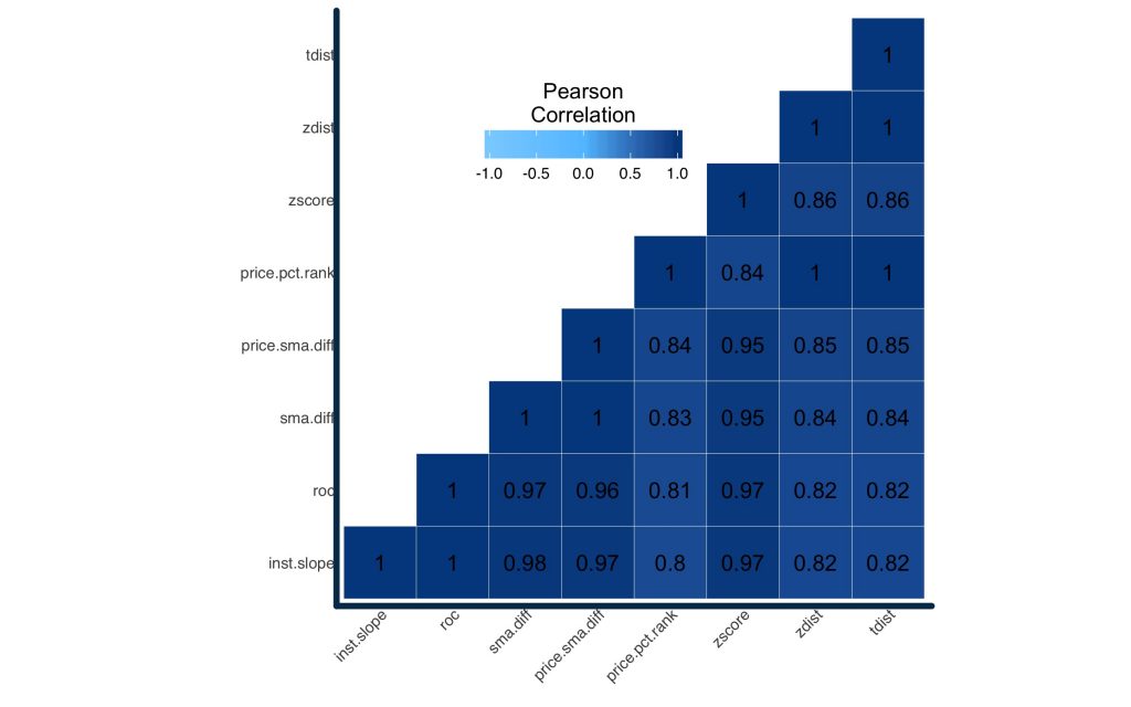
We know from all the statistics reported thus far that the different momentum indicators, with all the various combinations, offer different results, in some cases quite different. But just how different are these indicators, statistically speaking? In Figure 40 we have averaged the daily returns of all 16,116 combinations for correlation analysis.
Figure 41. Pairwise Correlations among Momentum Methodologies
Source: Global Financial Data, CSI Data, ReSolve Asset Management
The correlations run from a minimum of 0.8 (between the Price Percentile Rank and the Instantaneous Slope), to a high of .9999 between the Instantaneous Slope and Total Return ROC (note: these methods are mathematically almost identical). The average pairwise correlation across strategies is 0.923.
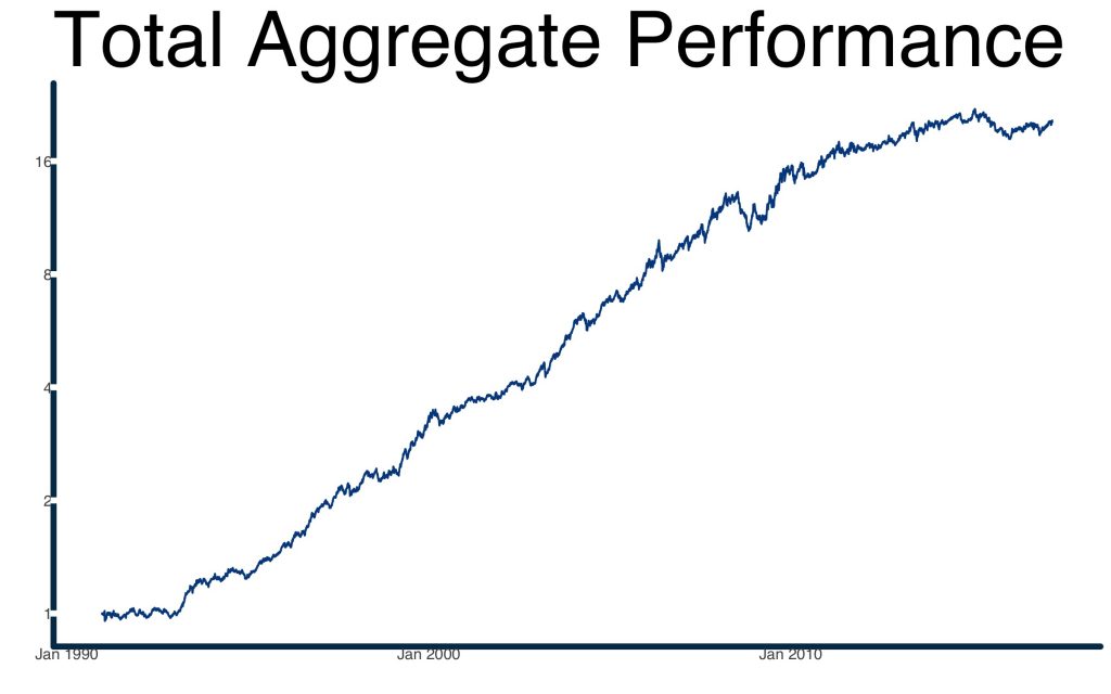
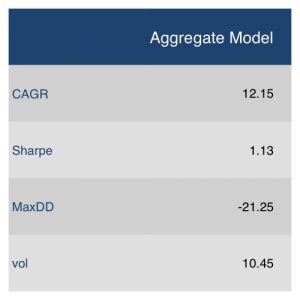
Figure 42. Aggregate Performance of all 128,928 Simulation Variations.
Source: Global Financial Data, CSI Data, ReSolve Asset Management
It’s hard to imagine that a system composed of such highly-correlated strategies could offer an edge over any of the individual strategies. This is especially true given the fact that several of the methods produced results that were significantly worse than others. Despite this intuition, an aggregate index provides a material boost to risk-adjusted performance relative to even the best individual strategy. As Figure 41 shows, this hypothetical meta-momentum strategy delivers the highest Sharpe ratio, and lowest volatility, while offering very similar compound returns and drawdowns.
Even within a single factor, diversification works.
Price Momentum is a Useful Indicator. But what about Risk-Adjusted Momentum?
In our next article we will perform the same battery of testing on several risk-adjust momentum measures, such as Sharpe ratio, Omega ratio, and Sortino Ratio. Then, as we round the corner into article 4, we will introduce methods to optimize the weights of portfolio holdings in order to further improve absolute and risk-adjusted returns.
Disclaimer
Confidential and proprietary information. The contents hereof may not be reproduced or disseminated without the express written permission of ReSolve Asset Management Inc. (“ReSolve”). ReSolve is registered as an investment fund manager in Ontario and Newfoundland and Labrador, and as a portfolio manager and exempt market dealer in Ontario, Alberta, British Columbia and Newfoundland and Labrador. These materials do not purport to be exhaustive and although the particulars contained herein were obtained from sources ReSolve believes are reliable, ReSolve does not guarantee their accuracy or completeness. The contents hereof does not constitute an offer to sell or a solicitation of interest to purchase any securities or investment advisory services in any jurisdiction in which such offer or solicitation is not authorized.
Forward-Looking Information. The contents hereof may contain “forward-looking information” within the meaning of the Securities Act (Ontario) and equivalent legislation in other provinces and territories. Because such forward-looking information involves risks and uncertainties, actual performance results may differ materially from any expectations, projections or predictions made or implicated in such forward-looking information. Prospective investors are therefore cautioned not to place undue reliance on such forward-looking statements. In addition, in considering any prior performance information contained herein, prospective investors should bear in mind that past results are not necessarily indicative of future results, and there can be no assurance that results comparable to those discussed herein will be achieved. The contents hereof speaks as of the date hereof and neither ReSolve nor any affiliate or representative thereof assumes any obligation to provide subsequent revisions or updates to any historical or forward-looking information contained herein to reflect the occurrence of events and/or changes in circumstances after the date hereof.
General information regarding returns. Performance data prior to August, 2015 reflects the performance of accounts managed by Dundee Securities Ltd., which used the same investment decision makers, processes, objectives and strategies as ReSolve has used since it became registered and commenced operations in August, 2015. Records that document and support this past performance are available upon request. Performance is expressed in CAD, net of applicable management fees. Indicated returns of one year or more are annualized. Past performance is not indicative of future performance.
General information regarding the use of benchmarks. The indices listed have been selected for purposes of comparing performance with widely-known, broad-based benchmarks. Performance may or may not correlate to any of these indices and should not be considered as a proxy for any of these indices. The S&P/TSX Composite Index (Net TR) (“S&P TSX TR”) is the headline index and the principal broad market measure for the Canadian equity markets. The Standard & Poor’s 500 Composite Stock Price Index (“S&P 500”) is a capitalization-weighted index of 500 stocks intended to be a representative sample of leading companies in leading industries within the U.S. economy.
General information regarding hypothetical performance and simulated results. These results are based on simulated or hypothetical performance results that have certain inherent limitations. Unlike the results in an actual performance record, these results do not represent actual trading. Also, because these trades have not actually been executed, these results may have under- or over-compensated for the impact, if any, of certain market factors, such as lack of liquidity. Simulated or hypothetical trading programs in general are also subject to the fact that they are designed with the benefit of hindsight. No representation is being made that any account or fund managed by ReSolve will or is likely to achieve profits or losses similar to those being shown. The results do not include other costs of managing a portfolio (such as custodial fees, legal, auditing, administrative or other professional fees). The contents hereof has not been reviewed or audited by an independent accountant or other independent testing firm. More detailed information regarding the manner in which the charts were calculated is available on request. Any actual fund or account that ReSolve manages will invest in different economic conditions, during periods with different volatility and in different securities than those incorporated in the hypothetical performance charts shown. There is no representation that any fund or account will perform as the hypothetical or other performance charts indicate.
General information regarding the simulation process. The systematic model used historical price data from Exchange Traded Funds (“ETFs”) representing the underlying asset classes in which it trades. Where ETF data was not available in earlier years, direct market data was used to create the trading signals. The hypothetical results shown are based on extensive models and calculations that are available for any potential investor to review before making a decision to invest.
© ReSolve Asset Management
Read more commentaries by ReSolve Asset Management
![\[T.R.Momentum=\frac{AdjPrice_t}{AdjPrice_{t-n}}-1\]](/images/content_image/data/5f/5f9710bea6bbc2bde0182aa63ba95fa2)
![\[SMA.Differential=\frac{SMA_{n/10}}{SMA_N}-1\]](/images/content_image/data/81/81762e29b6547b4c4dda017d4158f462)
![\[Price.to.SMA.Differential=\frac{AdjPrice_t}{SMA_n}-1\]](/images/content_image/data/17/17ec362bbc47f6cca647f46990899348)
![\[SMA.Inst.Slope=\frac{SMA_{n,t}}{SMA_{n,(t-1}}-1\]](/images/content_image/data/bf/bfef77ede087952f2459380ca9eef23b)
![\[(Rank(P_t, P_1,..,P_t)/t)*100\]](/images/content_image/data/6a/6aa514866fa693a5ef1864f1e1a76b12)
![\[ZScore=\frac{log(P_t) - \overline{log(P))}}{\sigma_{log(P)}}\]](/images/content_image/data/a4/a4e36f51d0f46a6a15be3a2a1051aa5f)
![\[ZDist=\phi(ZScore)\]](/images/content_image/data/60/60842224941e3091cab3662389bcfb23)
![\[TDist=\phi_t \frac{(P_t-\overline{log(P))}}{\sigma_{log(P)}/\sqrt{n}}\]](/images/content_image/data/2c/2c1dd8031a57098a09d487580df66db4)